
 Riskese
Do you speak riskese? Citizens of Japan speak Japanese, lawyers speak legalese, and leading investment advisors, casino statisticians and insurance actuaries speak “Riskese.” This is a self-created word for the essential language of investing and I use it to discuss topics of risk, return, statistical significance and time. Returns and risk go hand in hand. You cannot expect high returns without taking risk. People are perfectly comfortable talking about the returns portion of the investment process, but how squeamish do they get when they realize they will lose money on their investments? After the decline of 2008, people are far more aware of this possibility, but they are still looking for that perfect investment with small risk and big returns. People are also still looking for a weight loss pill that will allow them to continue eating country fried steak, massive cinnamon buns and ice cream on a regular basis. Neither exists.
One of the primary deterrents to investors earning market rates of returns is their lack of understanding of the relationship between risk and return. The natural tendency of investors is to want returns without the risk. Because risk is the source of returns, investors would be better served to be more concerned with the risk level of their investments.
The overall concept of the risk/return relationship is that when risk increases, the expected return on the asset should also increase as a result of an expected risk premium.

Blaise Pascal
Modern finance began with the realization that risk needed to be measured and managed. In 1654, French mathematicians Blaise Pascal and Pierre de Fermat tried to predict the future outcome of a game of chance. Their questions led to Pascal’s Theory of Probability, which quantifies the numerical likelihood of future events. Pascal’s Triangle was the foundation for learning how to manage the uncertainty of future outcomes, such as investment returns.
Every investment carries an expected return. The risk of an investment is quantified by the degree to which the returns of the investment deviate from the average return during specific periods of time. Higher risk investments carry a wider range of short-term outcomes but also carry higher expected returns, compensating investors for withstanding short-term volatility. In contrast, investments that have had a narrow range of outcomes over long periods of time are expected to provide more consistent returns with the trade-off of lower returns. For example, an all-bond index portfolio has provided a small but consistent return, while an all-equity index portfolio has provided a larger but more erratic return. Higher expected returns are the reward for an investor’s willingness to accept this volatility. In other words, risk is the source of returns and, therefore, should be embraced in appropriate doses.
An effective and common method to measure the deviation of investment returns from the average is the standard deviation of returns. Standard deviation provides a statistical measure of historical volatility and sets forth a distribution of the ranges of probable outcomes. In investing, measuring standard deviation of returns shows the extent to which returns (daily, monthly or annual) are distributed around the average return, estimating a range of probable outcomes and establishing a framework of risk and return trade-offs.
The normal distribution in the form of a bell-shaped curve shown in Figure 8-1 illustrates the concept of standard deviation. The curve represents a set of outcomes. In this case, let’s say the outcomes are the monthly returns of an investment. The yellow area covered in one standard deviation away from the average in both directions accounts for approximately 68% of the outcomes in a period. The area within two standard deviations from the average, the yellow and green shaded areas, accounts for 95.6% of outcomes, and the area up to three standard deviations away from the average-illustrated by the yellow, green and orange shaded areas-accounts for 99.7% of all outcomes. The higher an investment’s standard deviation, the greater the chance that future returns will lie farther away from the average return.
Figure 8-1(permalink)
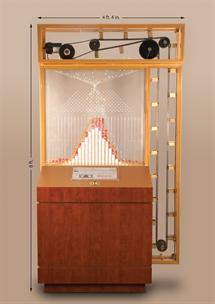 IFA's Probability Machine
Francis Galton, an English mathematician who was an expert in many scientific fields, created his “Quincunx” machine to demonstrate how a normal distribution is formed through the occurrence of multiple random events. He expressed his fascination with this phenomenon by stating, “I know of scarcely anything so apt to impress the imagination as the wonderful form of cosmic order expressed by the ‘Law of Frequency of Error.’ It reigns with serenity… amidst the wildest confusion. The huger the mob, and the greater the apparent anarchy, the more perfect is its sway. It is the supreme law of Unreason. Whenever a large sample of chaotic elements are taken in hand and marshalled in the order of their magnitude, an unsuspected and most beautiful form of regularity proves to have been latent all along.”1
I commissioned the creation of a large, museum-quality Probability Machine to educate investors about the probability of outcomes that result from a series of random events. The machine helps to portray order in the midst of seeming chaos that is the random walk of Wall Street. In the stock market, random events are the news stories about a company or about capitalism in general, and the resulting prices of securities. The random drop of the beads, starting with a central point of a fair price, simulates a series of fair prices, ultimately forming a normal distribution in the shape of a bell curve. The distribution of the beads bears a strong resemblance to the distribution of monthly returns shown in red bars behind the beads, also shown in Figure 8-2, reflecting 600 monthly returns (50 years) for an all-equity index portfolio. Like the Probability Machine’s normal distribution, the portfolio carries a wide range of outcomes or a high standard deviation. It maintains an approximate normal distribution that accumulates to an average 1.14% monthly fair return over 600 months, but with a standard deviation of 4.67%, which is a high level of short-term volatility. The display of the beads that have randomly fallen, and yet consistently form a bell curve approximating the returns of a full equity portfolio is so powerful, I created a desktop version of the machine that is available worldwide. It is called “The Random Walker.”
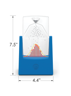
Figure 8-2(permalink)
Note the comparison to Figure 8-3, which shows a lower-risk index portfolio comprised of 90% fixed-income funds and 10% stock funds with a narrow range of outcomes. The 100% stock fund index portfolio in Figure 8-2 experienced greater price swings but had higher returns. Over the simulated 50-year period, a dollar invested in the low-risk index portfolio would have grown to $18.50, while a dollar invested in the higher risk index portfolio would have grown to $320.48. This historical data supports the presumption that investors who have the capacity to hold higher risks are expected to earn substantially higher returns.
Figure 8-3(permalink)
Higher expected returns are the result of higher risk, but not all risks are rewarded at the same rate. Financial economists have long sought to identify the factors that explain stock market returns. With the help of CRSP, substantial progress has been made. In Step 2, I discussed Nobel Laureate William Sharpe and his Capital Asset Pricing Model (CAPM). This model explains approximately 70% of all stock portfolio returns. CAPM enabled investors to quantify expected returns based on how investments fluctuate relative to the market as a whole. It concluded that investments which fluctuate more than the market, as a whole, carry more risk than the market, and therefore, should also carry higher expected returns. Sharpe asserted however, that some investments carry increased risk without providing the trade-off of higher expected returns. To clarify, he divided risk into two categories: systematic and unsystematic.
Figure 8-4(permalink)
The entire market is exposed to unavoidable systematic risk, such as war, recession, inflation, and government intervention. In contrast, unsystematic risk refers to threats specific to individual companies, such as lawsuits, fraud and competition. A summary of these different risks is presented in the top portion of Figure 8-4. Systematic risk, or the risk of investing in capitalism itself, has rewarded investors with an approximate 9.8% total U.S. market annualized return over the last 90 years (8.18% above the risk-free rate). However, an investment in unsystematic risk, such as buying individual stocks, does not increase expected returns. Unsystematic risk should be avoided through diversification, thereby maximizing portfolio efficiency and expected returns at each level of risk.
Figure 8-5(permalink)
Figure 8-5 illustrates the lack of increased expected returns when investors accept the additional concentrated and unsystematic risk of individual stocks relative to their designated index. The additional risk of buying individual stocks does not increase expected returns.
Even when all non-compensated risk has been eliminated from a portfolio, an investor cannot escape the systematic risks inherent in the market itself. As previously mentioned, history shows an investment in the U.S. market as a whole has delivered about 9.8% a year on average for the last 90 years, but not without substantial uncertainty. Risk and return go hand-in-hand. To obtain greater stock returns, the trade-off is suffering significant short-term volatility, such as that investors experience first-hand every day, with about 49% of daily returns being negative.
Sharpe’s CAPM was widely held as the explanation of equity returns until 1992 when Nobel Laureate Eugene Fama and Kenneth French introduced their Fama/French Three-Factor Model, identifying market, size and value as the three factors that explain as much as 96% of the returns of diversified stock portfolios. Fama and French analyzed the CRSP database back to 1962 to determine that equity returns can be explained by a portfolio’s exposure to the market as a whole, as well as the exposure to small and value companies. Their data show that small and value companies carried higher risk and that risk was rewarded. These small and value excess returns had shown to carry long-term persistence, but are not consistent in short periods of time. More than 90 years of risk and return data confirm their results.
Fama and French later expanded their model to include fixed income, identifying term and default as two additional risk factors that explain returns for fixed income. Thus, a Five-Factor Model was created, as shown in Figure 8-6.
Figure 8-6(permalink)
The relationship that exists between these five risk factors and a portfolio’s expected return serves as a framework for designing investment portfolios. The five risk factors are portrayed on the following pages.
 Market
The first risk factor in the Fama/French Five-Factor Model is the “market risk factor” or the amount of an investor’s exposure to the overall stock market compared to risk-free investments, such as the 30-day T-Bill. Investors take on market risk through all of their different equity investments. Figure 8-7 plots the risk and return associated with the market risk factor for five allocations of the total U.S. stock market and U.S. Treasury bills. The highest market exposure, labeled 5, carries 100% exposure to the total U.S. market. The button labeled 0 is invested in 100% T-Bills. The chart reflects the differences in growth of $1 and annualized returns in the various market exposures over the 90-year period from January 1, 1928 through December 31, 2017.
Figure 8-7(permalink)
 Size
Size
The second risk factor in the Fama/French model is the “size risk factor,” referring to the level of a portfolio’s exposure to small company stocks. Small companies are more volatile and riskier than larger companies because they have less business diversification, fewer financial resources and greater uncertainty of earnings than their large counterparts.
The painting for the size factor contrasts General Electric with the small cap company Acme Packet. It is obvious that Acme is a riskier investment than GE, therefore the cost of capital for Acme and the expected return for its investors should be higher.
Figure 8-8 plots the risk and return of the S&P 500 Index and U.S. companies according to size over a 90-year period.
Figure 8-8(permalink)
 Value
Value
The third risk factor in the Fama/French model is the “value risk factor,” which refers to the amount of a portfolio’s exposure to value or low-priced stocks relative to their book value. Value is measured by the book-to-market (BtM) ratio. The book value of a company is an accounting term for its net worth, its assets minus its liabilities. The market value of a company is its price per share times the number of shares outstanding. Stocks with higher BtM ratios are considered value stocks while stocks with lower BtM ratios are considered growth stocks. Figure 8-9 plots the risk and return characteristics and the growth of $1 for the value risk factor for the five quintiles of the U.S. stock market from 1928 through 2017.
Figure 8-9(permalink)
 Term
Term
Fixed income is also an important component to an investment portfolio. Since stocks and bonds frequently move in opposite directions, holding low-volatility bonds provides good diversification and will therefore level out a portfolio’s performance by dampening stock volatility and providing short-term liquidity.
The “term (maturity) risk factor” refers to the difference in returns between long-term government bonds and short-term treasury bills. Longer-term bonds are riskier than shorter-term instruments and have yielded higher returns over the 90 years ending in 2017. Figure 8-10 shows six different fixed income allocations and their differences in risk and return.
Figure 8-10(permalink)
 Default
The last of the five risk factors is the “default risk factor,” which is associated with the credit quality of bonds. Instruments of lower credit quality are riskier than those of higher credit quality, thus yielding higher expected returns. Despite the downgrade of U.S. government debt by Standard & Poor’s that occurred in 2011, the market still assigns a higher default risk to corporations over the U.S. government. The default risk factor refers to the additional expected return of corporate bonds over government bonds. Figure 8-11 shows the strong relationship between risk, return and the growth of $1 as the probability of default increases.
Figure 8-11(permalink)
A summary of the average annual returns for all five risk factors is presented in Figure 8-12. Both the risk and average annual returns for all five risk factors are shown in Figure 8-13.
Figure 8-12(permalink)
Figure 8-13(permalink)
The research of Eugene Fama and Kenneth French serves as a guiding protocol for both individual and institutional investing. Their Multi-Factor Model has revolutionized how portfolios are constructed and analyzed, and was one of the primary reasons for Eugene Fama being awarded the 2013 Nobel Prize in Economics.
As you have learned, three-of-the-five factors apply to equities. The Three-Factor Model is an invaluable tool for asset allocation and portfolio analysis. In his own words, Eugene Fama explains the small-value story, among other subjects, in a November 2007 interview with The Region, a publication for the Federal Reserve Bank of Minneapolis. “So, small-cap stocks have higher average returns than large-cap stocks, and stocks with higher ratios of book value to market value have higher returns than low book-to-market stocks.” He continues, “Low book-to-market stocks tend to be growth stocks. High book-to-market stocks tend to be relatively more distressed; they’re what people call value stocks. That’s given rise to what the finance profession — academic as well as applied — calls the size premium and the value premium. The value premium tends to be bigger” he said. “So, our model has three factors. Every asset pricing model says you need the market in there. Then they differ on how many other things you need. The CAPM says you only need the market. We basically say a minimum of two other factors seem to be necessary. And these two do a pretty good job.”"2
See Appendix A (https://www.ifa.com/disclosures/)